Extracting irradiance from ray tracing with dedicated sensors in SunSolve

The ray-traced outputs reported by SunSolve have expanded to include irradiation, irradiance and absorbed energy density. The new outputs allow simulation of plane-of-array (POA) sensors and tracking of energy absorption in objects. This answers a wide range of detailed, and often highly requested, questions about PV systems in the real world.

Questions like, “How does the location or tilt of a pyranometer affect the irradiance it receives?”, “What is the spectral mismatch error between my pyranometer and my module?”, “How much energy will get absorbed in the plastic housing of a box attached to the tracker post?”, “How much energy reaches the plants on the ground under the array?” or even “What is the irradiance on the front and rear of the panel?” In this post we are going to take a look at one aspect of this upgrade, extracting irradiance from the ray tracing via a dedicated sensor.

Previous versions of SunSolve only reported POA irradiance from view-factor models (as part of a waterfall loss chart). The new upgrade allows objects in the scene to track their absorption during the ray tracing step. That absorption (which is solved for a limited wavelength range) is converted into irradiance using the broadband global horizontal irradiance in the weather file.¹ These objects can be placed across the whole panel, to measure the full area POA, or they can be added in discrete locations. They can track with the panels or remain fixed. You can even add angles to them to check what will happen when the sensors are not mounted perfectly in the real world.

Figure 1: Example of plane-of-array sensors modelled in SunSolve, placed across a two-panel-in-portrait (2P) tracker.

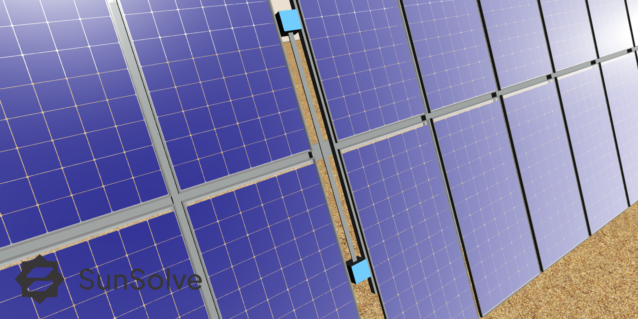
Simulating POA sensors in SunSolve

It is common practice to use thermopile pyranometers to monitor the solar resource at a site. These may be held horizontally to sample the global horizontal irradiance (GHI), or they may be mounted alongside the panels to sample the irradiance that is incident on the tilted plane (GTI or POA). These sensors are calibrated to report irradiance representative of the sun’s full spectrum.² They are also designed to capture the irradiance irrespective of the incidence angle. This is different to a typical crystalline silicon module which only collects photons between 300 nm and 1200 nm and which has an angular dependence to its absorption caused by the air-glass interface.

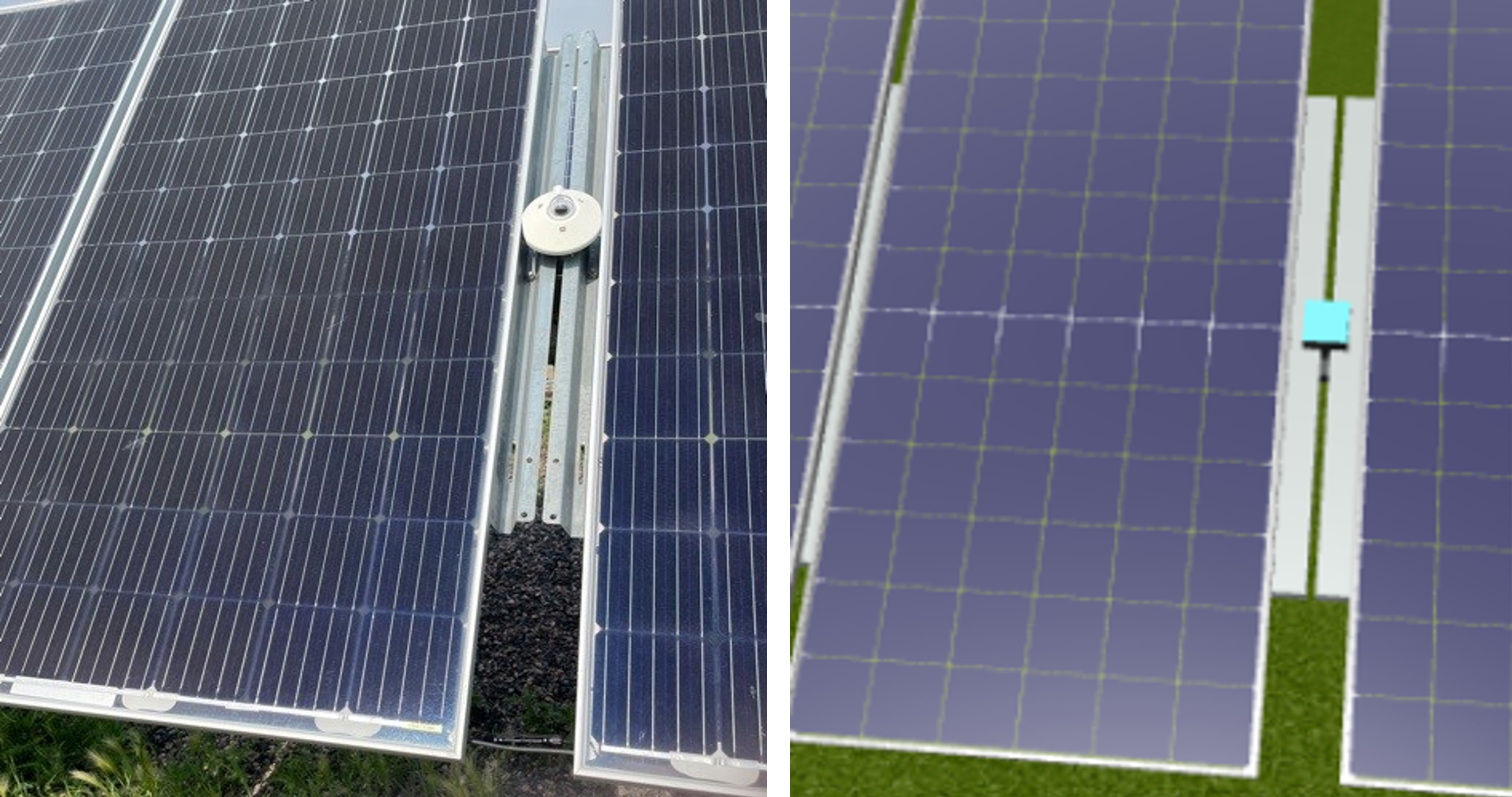
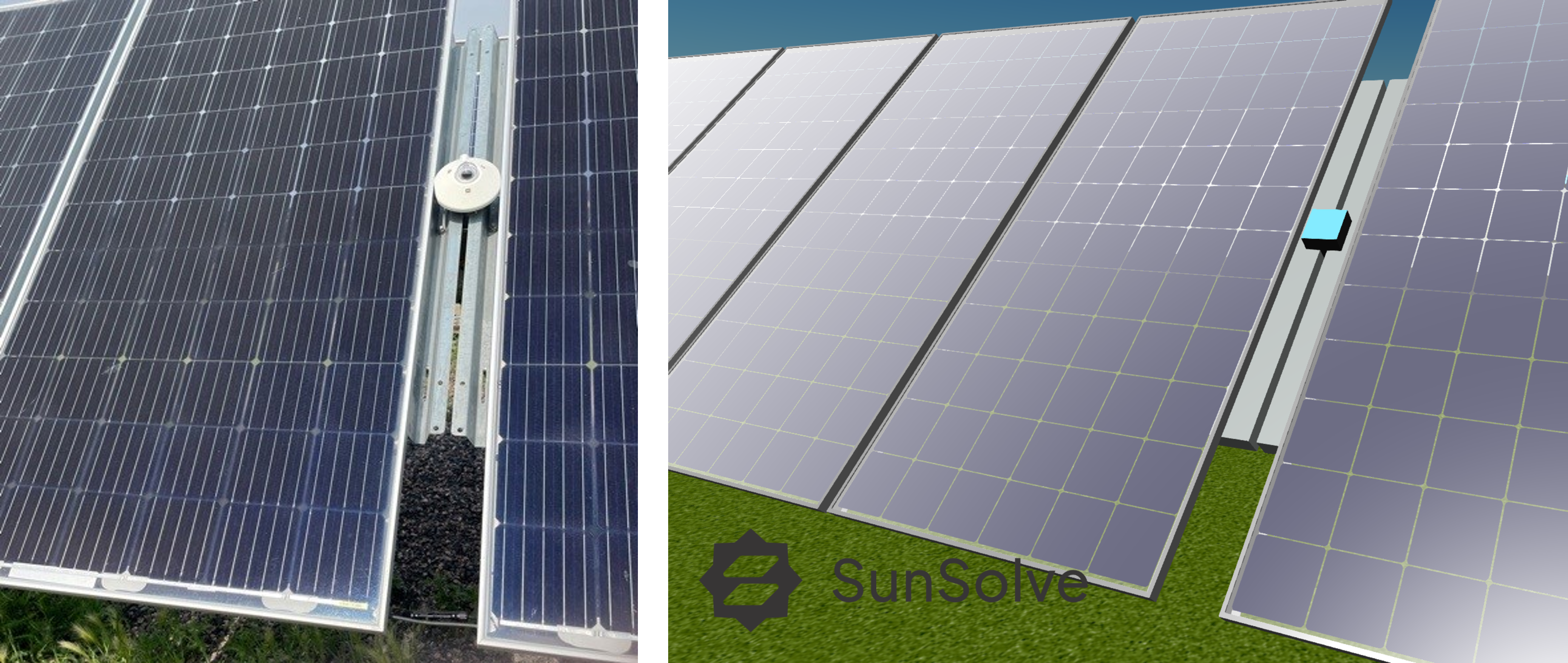
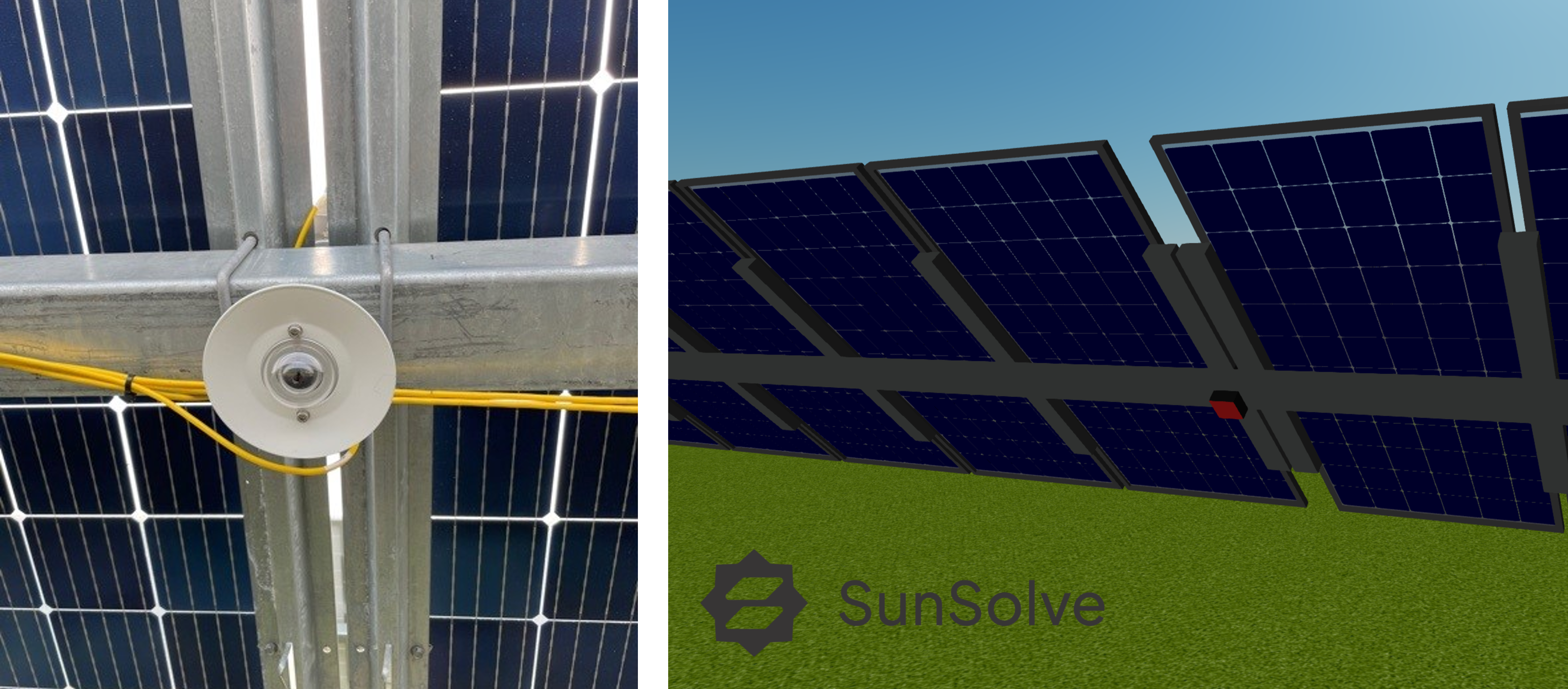
To demonstrate how they can be modelled in SunSolve we will make use of a site run by FTC Solar in collaboration with NREL. You can see the site details in our collaborative paper and related video from the time. Included in the metrology were front- and rear-facing POA sensors that were well maintained and recently calibrated. The images that follow both show a site photo on the left, and the re-creation of it in SunSolve on the right. The sensors in SunSolve detect from a front face (light blue) and a rear face (red).

Figure 2: The front-facing POA sensor at the FTC Solar / NREL site (left) and its re-creation in SunSolve (right), where the front detection face is shown in light blue.

Figure 3: The rear-facing POA sensor at the site (left) and its re-creation in SunSolve (right), where the rear detection face is shown in red.

On one of the measurement days a white tarpaulin was placed on the ground under the modules and sensors. This allowed a controlled, uniform albedo during the measurement period. The comparison between SunSolve and the measurements from that day is shown below. It demonstrates good agreement between the ray tracing result and measurements from the field. The only free variable used in the fitting was the fixed value of albedo (set to 59%) which was unfortunately not measured on site.

Figure 4: Front-side POA irradiance over the measurement day, comparing the SunSolve ray tracing result against the field measurement.

Figure 5: Rear-side POA irradiance over the measurement day, comparing the SunSolve ray tracing result against the field measurement.

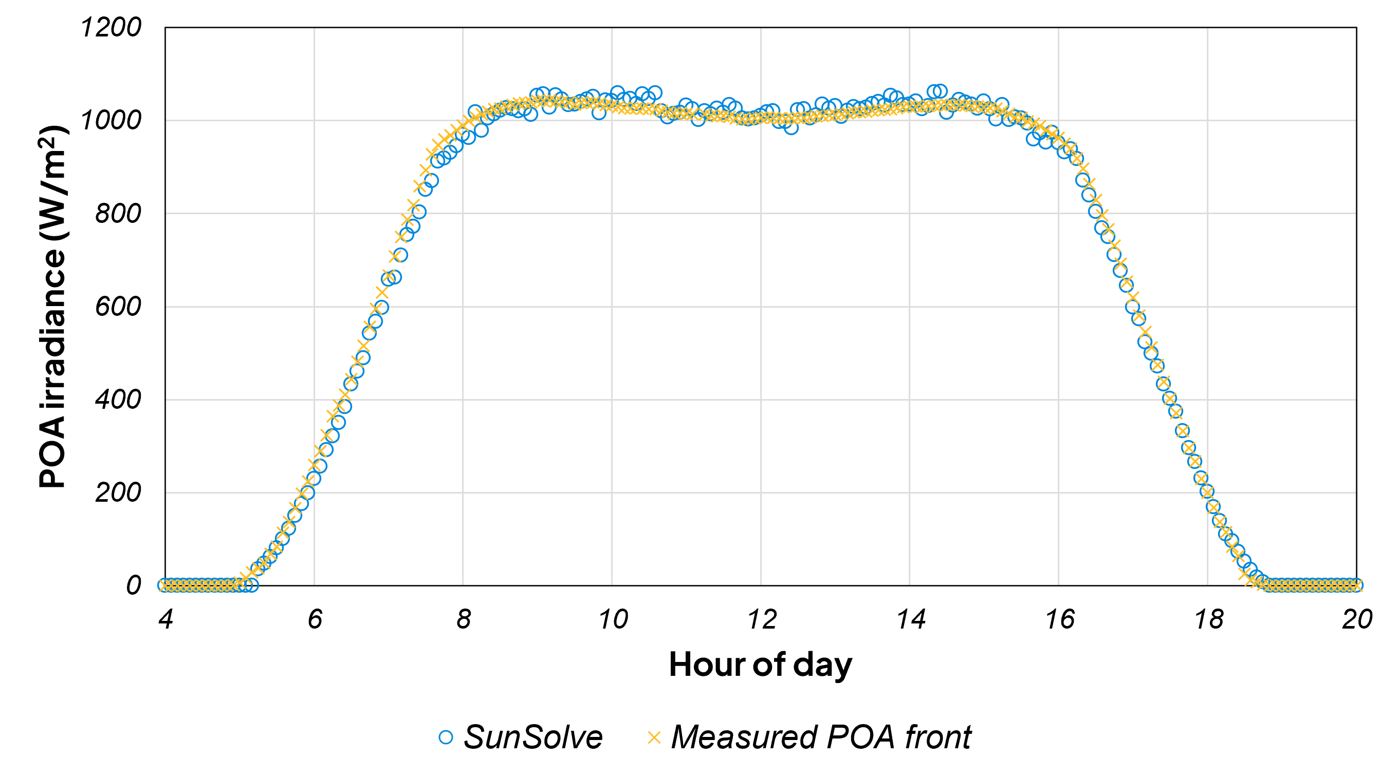
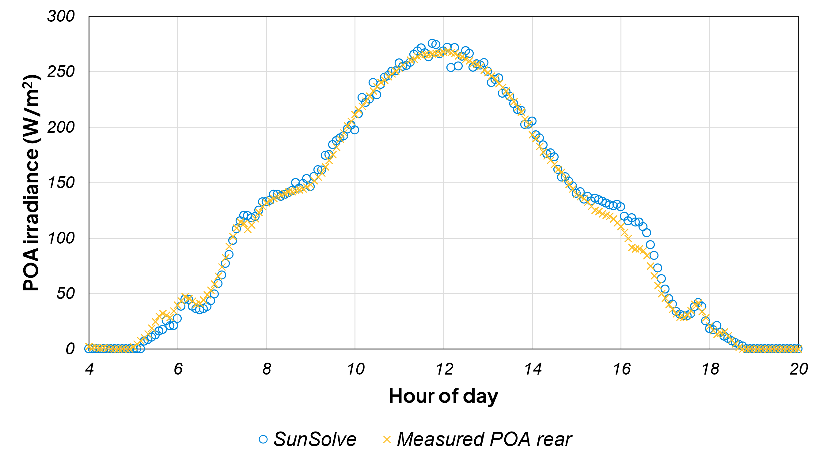
The 5-minute time steps reveal fine-scale variations. On the rear side, these variations correspond to shadows and bands of light cast by the two neighbouring rows as they move across the ground and as the sensor’s area of detection changes.

Simulating GHI measurements in SunSolve

At first, it might seem strange to try and simulate a GHI sensor. Particularly since the GHI is an input to the simulation. However, you would be surprised how many irradiance-based software packages out there do not faithfully reproduce the GHI. Running this sort of simulation is a great validation test to apply. It can also be handy when interpreting measured data.

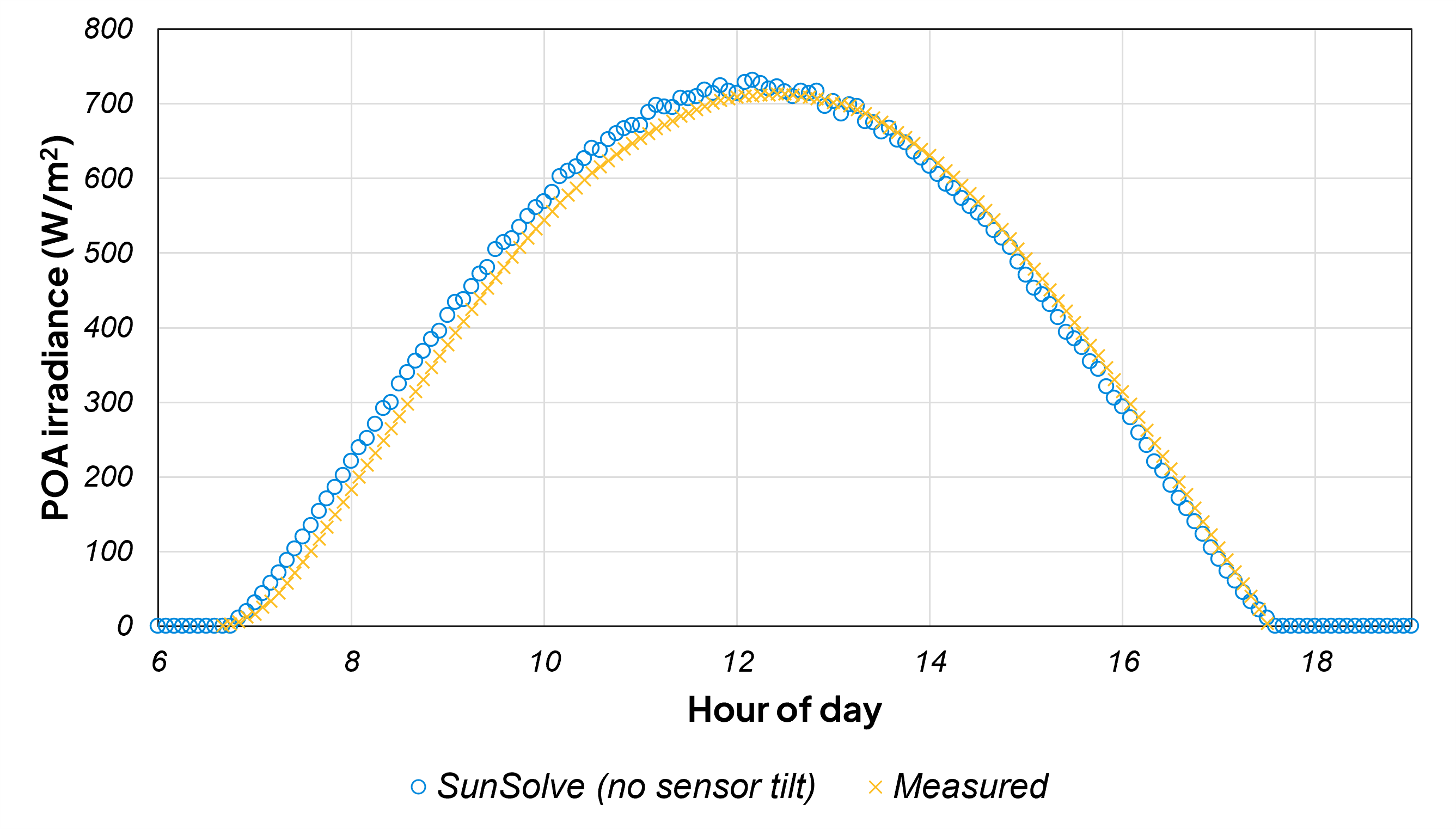
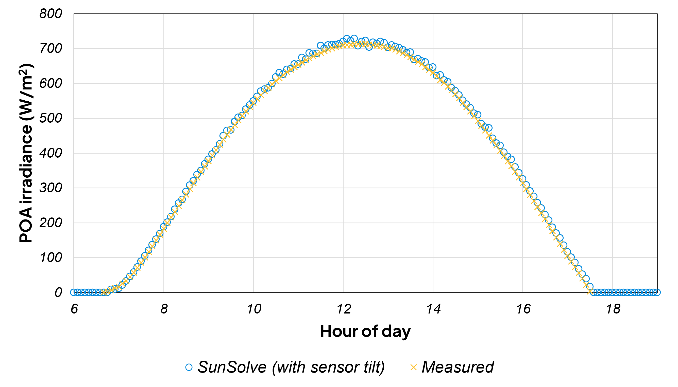
For example, Figure 6 shows a measurement taken with a front-side POA sensor held flat throughout a sunny day³, alongside the SunSolve simulation result for a flat sensor. Figure 7 compares the same measurement with a simulation of a sensor mounted at an angle of 2.5° to the east. Notice that the results in Figure 7 align more closely. This was likely caused by a very slight offset in how the POA sensor was mounted in the field.

Figure 6: GHI measured with a flat front-side POA sensor compared against the SunSolve simulation of a flat sensor.

Figure 7: The same measurement compared against a SunSolve simulation of a sensor tilted 2.5° to the east, showing the improved alignment that points to a slight mounting offset in the field.

The ray tracing results demonstrated in this blog post made use of SunSolve’s direct ray tracing mode. In this mode SunSolve calculates the optical solution at every sun position, once for the direct light and once for the diffuse light. This is typically applied to smaller time spans (e.g. a single day of 5-minute steps) and is used when studying system performance in detail. It differs from the mode used for annual solving in which discrete solar arcs and interpolation are used.

You can place a sensor almost anywhere in the scene. Flat on the ground, alongside the panel, or tilted to match an imperfect real-world mount. This is the kind of detail that is easy to overlook, and it is exactly what standard yield tools tend to miss. It is one more way SunSolve lets you see what others can’t.

Interested in fully ray-traced POA sensor simulations? Contact us for a fully supported trial.

This was supported by funding from the Australian Renewable Energy Agency (ARENA). The views expressed herein are not necessarily the views of the Australian Government, and the Australian Government does not accept responsibility for any information or advice contained herein.